用 Python 自學資料科學與機器學習入門實戰：Pandas 基礎入門

2017年10月11日 · 閱讀時間約 12 分鐘

站長

Python 資料科學系列教學

本文是 Python 資料科學與機器學習系列 的第三篇文章：

如何使用 Python 學習機器學習（Machine Learning）

本系列文章將透過 Python 及其資料科學生態系（Numpy、Scipy、Pandas、Scikit-learn、Statsmodels、Matplotlib、Scrapy、Keras、TensorFlow 等）來系統性介紹資料科學和相關的知識，透過 Python 帶領讀者進入資料科學的世界和機器學習的世界。在這個單元中我們將介紹 Pandas 這個基於 Numpy 的資料處理和分析神兵利器。

事實上，真實世界並非如此美好，大部分資料分析的工作時間有很大一部分都是在處理髒資料，希望讓資料可以符合模型輸入的需求，而 Pandas 正是扮演這個資料預處理和資料清洗的核心角色，是 Python 在和 R 爭奪資料科學第一程式語言霸主時的生力軍，接下來我們將介紹 Pandas 核心功能和資料的操作方式。

如何使用 Python 學習機器學習（Machine Learning）

Pandas 核心功能介紹

創建資料結構

在 Pandas 中主要有兩大資料結構：Series、DataFrame，與 Numpy 中的 ndarray 比較不同的是 Pandas DataFrame 可以存異質資料（不同資料型別）。

Series 類似於 Python 本身的 list 資料結構，不同的是每個元素有自己的 index（可以自己命名）：

%matplotlib inline
# 引入 numpy 和 pandas 模組
import numpy as np 
import pandas as pd
s1 = pd.Series([1, 3, 5, np.nan, 6, 8]) # 使用 Python lits 產生 Series，其中包含一個值為 NaN 

print(s1)

0 1.0 1 3.0 2 5.0 3 NaN 4 6.0 5 8.0 dtype: float64

s2 = pd.Series(np.random.randint(2, size=[3])) # 使用 np.random.randint 產生 3 個 0-2（不含 2）的數組

print(s2)

0 1 1 1 2 1 dtype: int64

DataFrame 可以使用 np.random.randn 產生值來創建，也可以使用 Python dict 進行創建：

# 產生 20170101-20170106 的值，DatetimeIndex(['2017-01-01', '2017-01-02', '2017-01-03', '2017-01-04', '2017-01-05', '2017-01-06'], dtype='datetime64[ns]', freq='D')
dates = pd.date_range('20170101', periods=6)

# 產生 row6,column4 個 standard normal distribution 隨機值，使用 ABCD 當 columns，使用 dates 當 index
df0 = pd.DataFrame(np.random.randn(6,4), index=dates, columns=list('ABCD')) 
print(df0)

A B C D 2017-01-01 1.112542 -0.142577 0.832830 -2.755133 2017-01-02 -0.218838 -0.304488 1.437599 -0.402454 2017-01-03 0.295245 -0.786898 -1.231896 -0.224959 2017-01-04 -0.346745 -1.582944 -0.464175 -0.410576 2017-01-05 0.163782 0.948795 -0.420505 -0.641032 2017-01-06 0.515806 -0.935421 -0.701349 -0.820109

# 使用 dict 來創建 DataFrame
teams = ['Web', 'Mobile', 'Data']
nums = [12, 14, 34]
rd_team_dict = {
                'teams': teams,
                'nums': nums
}
rd_team_df = pd.DataFrame(rd_team_dict)

print(rd_team_df)

nums teams 0 12 Web 1 14 Mobile 2 34 Data

觀察資料

# 觀察資料型態、結構、內容值
df = pd.DataFrame({ 'A' : 1.,
                    'B' : pd.Timestamp('20170102'),
                    'C' : pd.Series(1,index=list(range(4)),dtype='float32'),
                    'D' : np.array([3] * 4,dtype='int32'),
                    'E' : pd.Categorical(["test","train","test","train"]),
                    'F' : 'foo' })

# 印出內容值資料型別
print(df.dtypes)

A float64 B datetime64[ns] C float32 D int32 E category F object dtype: object

# 印出資料維度
print(df.shape)

(4, 6)

# 印出每行資料長度
print(len(df))

# 印出 DataFrame 資料概況
print(df.info())

<class 'pandas.core.frame.DataFrame'> Int64Index: 4 entries, 0 to 3 Data columns (total 6 columns): A 4 non-null float64 B 4 non-null datetime64[ns] C 4 non-null float32 D 4 non-null int32 E 4 non-null category F 4 non-null object dtypes: category(1), datetime64ns, float32(1), float64(1), int32(1), object(1) memory usage: 180.0+ bytes None

# 印出基本敘述統計數據
print(df.describe())

A C D count 4.0 4.0 4.0 mean 1.0 1.0 3.0 std 0.0 0.0 0.0 min 1.0 1.0 3.0 25% 1.0 1.0 3.0 50% 1.0 1.0 3.0 75% 1.0 1.0 3.0 max 1.0 1.0 3.0

# 印出首 i 個數據
print(df.head(2))

A B C D E F 0 1.0 2017-01-02 1.0 3 test foo 1 1.0 2017-01-02 1.0 3 train foo

# 印出尾 i 個數據
print(df.tail(2))

A B C D E F 2 1.0 2017-01-02 1.0 3 test foo 3 1.0 2017-01-02 1.0 3 train foo

# 印出 index 值
print(df.index)

Int64Index([0, 1, 2, 3], dtype='int64')

# 印出 columns 值
print(df.columns)

Index(['A', 'B', 'C', 'D', 'E', 'F'], dtype='object')

# 印出 values 值
print(df.values)

[[1.0 Timestamp('2017-01-02 00:00:00') 1.0 3 'test' 'foo'] [1.0 Timestamp('2017-01-02 00:00:00') 1.0 3 'train' 'foo'] [1.0 Timestamp('2017-01-02 00:00:00') 1.0 3 'test' 'foo'] [1.0 Timestamp('2017-01-02 00:00:00') 1.0 3 'train' 'foo']]

# 印出轉置 DataFrame
print(df.T)

0 1 2
A 1 1 1
B 2017-01-02 00:00:00 2017-01-02 00:00:00 2017-01-02 00:00:00
C 1 1 1
D 3 3 3
E test train test
F foo foo foo

3
A 1
B 2017-01-02 00:00:00
C 1
D 3
E train
F foo

# sort by the index labels。axis=0 使用 index 進行 sort，axis=1 使用 columns 進行 sort。ascending 決定是否由小到大
print(df.sort_index(axis=0, ascending=False))

A B C D E F 3 1.0 2017-01-02 1.0 3 train foo 2 1.0 2017-01-02 1.0 3 test foo 1 1.0 2017-01-02 1.0 3 train foo 0 1.0 2017-01-02 1.0 3 test foo

# sort by the values of columns
print(df.sort_values(by='E'))

A B C D E F 0 1.0 2017-01-02 1.0 3 test foo 2 1.0 2017-01-02 1.0 3 test foo 1 1.0 2017-01-02 1.0 3 train foo 3 1.0 2017-01-02 1.0 3 train foo

選取資料

# 選取值的方式一般建議使用 1. loc, 2. iloc, 3. ix
# label-location based 行列標籤值取值，以下取出 index=1 那一欄，[列, 行]
print(df.loc[0])

A 1 B 2017-01-02 00:00:00 C 1 D 3 E test F foo Name: 0, dtype: object

# iloc 則通過行列數字索引取值，[列，行]
print(df.iloc[0:3, 1:2])

B 0 2017-01-02 1 2017-01-02 2 2017-01-02

# 兼容 loc 和 iloc
print(df.ix[0, 'B'])

2017-01-02 00:00:00

# 兼容 loc 和 iloc
print(df.ix[1, 3])

# 布林取值，取出 A 行大於 0 的資料
print(df[df.A > 0])

A B C D E F 0 1.0 2017-01-02 1.0 3 test foo 1 1.0 2017-01-02 1.0 3 train foo 2 1.0 2017-01-02 1.0 3 test foo 3 1.0 2017-01-02 1.0 3 train foo

# 產生 Series 值
s1 = pd.Series([1,2,3,4,5,6], index=pd.date_range('20170102', periods=6))
print(s1)

2017-01-02 1 2017-01-03 2 2017-01-04 3 2017-01-05 4 2017-01-06 5 2017-01-07 6 Freq: D, dtype: int64

# 更新值
df.loc[:,'D'] = np.array([5] * len(df))
print(df)

A B C D E F 0 1.0 2017-01-02 1.0 5 test foo 1 1.0 2017-01-02 1.0 5 train foo 2 1.0 2017-01-02 1.0 5 test foo 3 1.0 2017-01-02 1.0 5 train foo

處理遺失資料

# 查缺補漏
df2 = pd.DataFrame(index=dates[0:4], columns=list(df.columns) + ['E'])

df2.loc[dates[0]:dates[1], :] = 1

# drop 掉 NaN 值
print(df2.dropna(how='any'))
# 補充 NaN 為 3
print(df2.fillna(value=3))
print(df2)

# 回傳 NaN 布林值 
print(pd.isnull(df2))

# inplace 為 True 為直接操作資料，不是操作 copy 副本
df2.dropna(how='any', inplace=True)

A B C D E F E 2017-01-01 1 1 1 1 1 1 1 2017-01-02 1 1 1 1 1 1 1 A B C D E F E 2017-01-01 1 1 1 1 1 1 1 2017-01-02 1 1 1 1 1 1 1 2017-01-03 3 3 3 3 3 3 3 2017-01-04 3 3 3 3 3 3 3 A B C D E F E 2017-01-01 1 1 1 1 1 1 1 2017-01-02 1 1 1 1 1 1 1 2017-01-03 NaN NaN NaN NaN NaN NaN NaN 2017-01-04 NaN NaN NaN NaN NaN NaN NaN A B C D E F E 2017-01-01 False False False False False False False 2017-01-02 False False False False False False False 2017-01-03 True True True True True True True 2017-01-04 True True True True True True True

資料操作

# 針對每一個值進行操作
df.apply(lambda x: x.max() - x.min())

A 2.696944 B 5.285329 C 1.948946 D 2.615037 dtype: float64

串接資料

# 串接資料

df = pd.DataFrame(np.random.randn(10, 4))
print(df)
pieces = [df[:3], df[3:7], df[7:]]
print(pieces)
print(pd.concat(pieces))

0 1 2 3 0 -0.171208 2.200967 0.385574 -0.481588 1 1.447335 1.756239 0.083053 0.255434 2 -0.508576 0.818774 -0.438210 -0.819860 3 1.704828 -0.329642 -1.059202 -0.820319 4 -1.792491 -0.761873 -1.090574 -0.484552 5 0.166621 1.704577 -1.613185 -0.391985 6 0.806292 0.699608 -1.768223 -1.081318 7 -1.168532 0.768302 0.831701 0.422367 8 0.065940 -0.038649 -0.060712 -0.500365 9 0.623535 0.558461 -0.956861 1.229675 [ 0 1 2 3 0 -0.171208 2.200967 0.385574 -0.481588 1 1.447335 1.756239 0.083053 0.255434 2 -0.508576 0.818774 -0.438210 -0.819860, 0 1 2 3 3 1.704828 -0.329642 -1.059202 -0.820319 4 -1.792491 -0.761873 -1.090574 -0.484552 5 0.166621 1.704577 -1.613185 -0.391985 6 0.806292 0.699608 -1.768223 -1.081318, 0 1 2 3 7 -1.168532 0.768302 0.831701 0.422367 8 0.065940 -0.038649 -0.060712 -0.500365 9 0.623535 0.558461 -0.956861 1.229675] 0 1 2 3 0 -0.171208 2.200967 0.385574 -0.481588 1 1.447335 1.756239 0.083053 0.255434 2 -0.508576 0.818774 -0.438210 -0.819860 3 1.704828 -0.329642 -1.059202 -0.820319 4 -1.792491 -0.761873 -1.090574 -0.484552 5 0.166621 1.704577 -1.613185 -0.391985 6 0.806292 0.699608 -1.768223 -1.081318 7 -1.168532 0.768302 0.831701 0.422367 8 0.065940 -0.038649 -0.060712 -0.500365 9 0.623535 0.558461 -0.956861 1.229675

合併資料

# 合併資料
left = pd.DataFrame({'key': ['foo', 'foo'], 'lval': [1, 2]})
right = pd.DataFrame({'key': ['foo', 'foo'], 'rval': [4, 5]})

print(pd.merge(left, right, on='key'))

key lval rval 0 foo 1 4 1 foo 1 5 2 foo 2 4 3 foo 2 5

新增資料

# 新增資料於最後
df = pd.DataFrame(np.random.randn(8, 4), columns=['A','B','C','D'])
print(df)
s = df.iloc[3]
print(df.append(s, ignore_index=True))

A B C D 0 1.780499 1.207626 0.631475 -1.747506 1 -0.603999 -2.364099 1.153066 0.504784 2 0.721924 0.199784 -0.158318 -0.882946 3 -0.378070 -0.379311 0.478997 0.271056 4 0.620888 -0.366262 -0.738695 -0.380854 5 -0.587604 -1.728096 0.279645 -0.927843 6 -0.916445 2.921231 -0.795880 0.867531 7 -0.373190 1.526771 0.136712 0.015765 A B C D 0 1.780499 1.207626 0.631475 -1.747506 1 -0.603999 -2.364099 1.153066 0.504784 2 0.721924 0.199784 -0.158318 -0.882946 3 -0.378070 -0.379311 0.478997 0.271056 4 0.620888 -0.366262 -0.738695 -0.380854 5 -0.587604 -1.728096 0.279645 -0.927843 6 -0.916445 2.921231 -0.795880 0.867531 7 -0.373190 1.526771 0.136712 0.015765 8 -0.378070 -0.379311 0.478997 0.271056

群組操作

# 群組操作
print(df.groupby(['A','B']).sum())

C D A B
-1.232691 0.489020 0.436602 -1.439868 -0.259460 -0.269874 1.655001 0.530137 -0.256261 -0.743254 0.128837 1.050430 0.015723 0.596866 -0.232503 1.247810 0.049633 -0.093130 0.895723 1.049938 0.458667 0.348883 -0.681931 -0.517437 1.446492 0.007736 0.208870 0.211517 2.357912 -0.187805 -0.376578 -0.459085

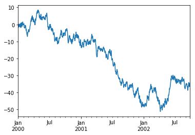
繪圖

# 印出圖表
ts = pd.Series(np.random.randn(1000), index=pd.date_range('1/1/2000', periods=1000))
ts = ts.cumsum()
ts.plot()

png

輸入/輸出

# 讀取檔案/輸出檔案，支援 csv, h5, xlsx 檔案格式
df.to_csv('foo.csv')
pd.read_csv('foo.csv')
df.to_excel('foo.xlsx', sheet_name='Sheet1')
print(pd.read_excel('foo.xlsx', 'Sheet1', index_col=None, na_values=['NA']))

A B C D 0 1.446492 0.007736 0.208870 0.211517 1 0.049633 -0.093130 0.895723 1.049938 2 -1.232691 0.489020 0.436602 -1.439868 3 -0.259460 -0.269874 1.655001 0.530137 4 0.015723 0.596866 -0.232503 1.247810 5 0.458667 0.348883 -0.681931 -0.517437 6 2.357912 -0.187805 -0.376578 -0.459085 7 -0.256261 -0.743254 0.128837 1.050430

總結

以上整理了一些 Pandas 核心功能和如何操作資料，接下來我們將介紹其他 Python 資料科學和機器學習生態系和相關工具。

延伸閱讀

（image via pydata、nbcnews）

Pandas 核心功能介紹

創建資料結構​

觀察資料

選取資料​

處理遺失資料​

資料操作​

串接資料​

合併資料​

新增資料​

群組操作​

繪圖​

輸入/輸出​

總結